1 Introduction to R

1.1 Installation

R is a free software environment for statistical computing and graphics. It compiles and runs on a wide variety of UNIX platforms, Windows and macOS. To help you write code in R, RStudio is a free application that makes the task significantly easier. To get started, you need to acquire your own copies of these two programs. If you already have R and Rstudio installed on your computer, it is a good idea to update to the latest versions by following the same step since some of the packages employed later work only with recent versions of this software.

1.1.1 Installation of R

We start with the installation of R. The essential files for installation and packages can be found on The Comprehensive R Archive Network (CRAN) website, http://cran.r-project.org/, as shown in Figure 1.1 below.

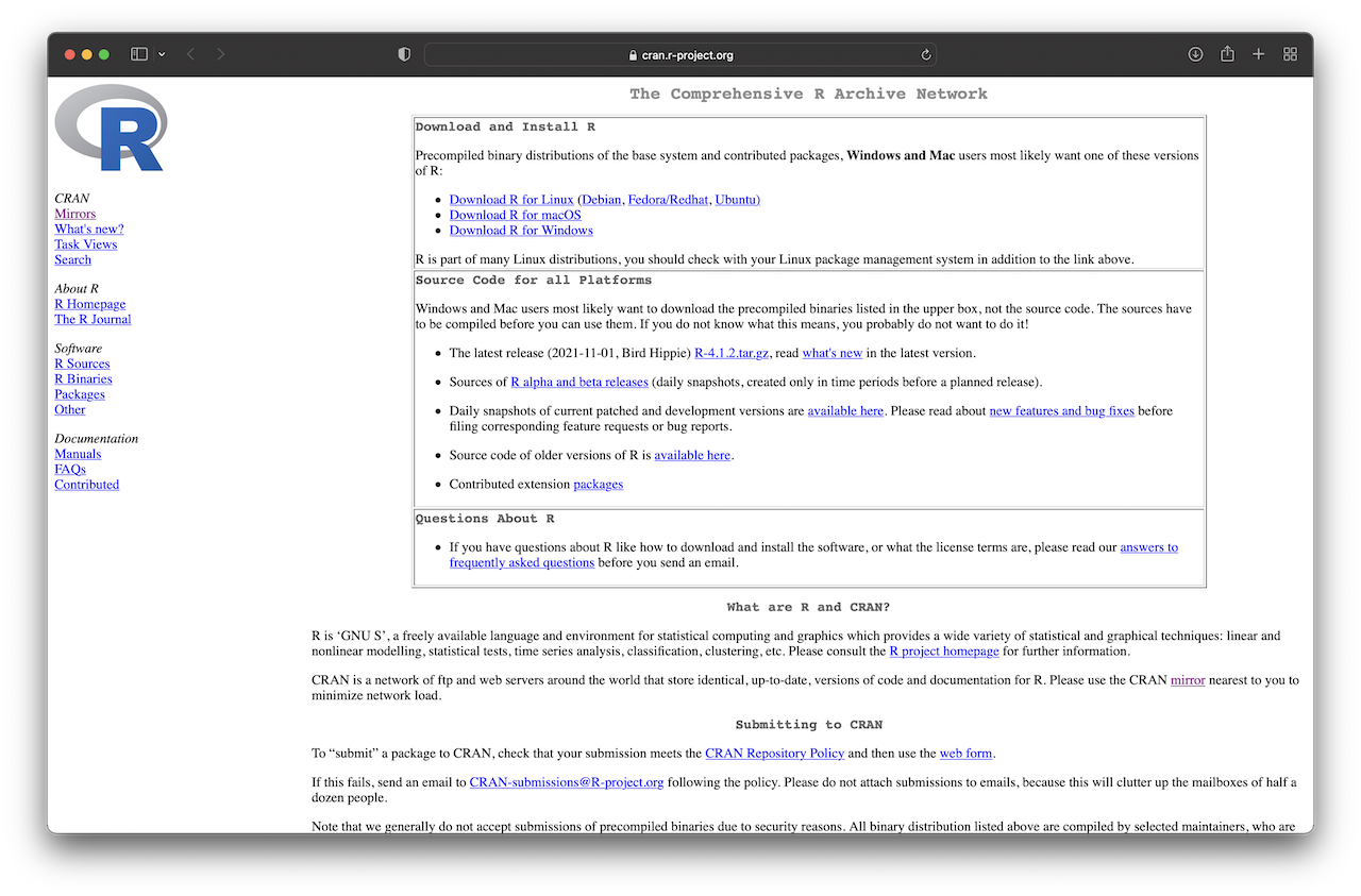
Figure 1.1: CRAN webpage.

For Windows users, click “Download R for Windows.” Then, you will obtain a screen similar to Figure 1.2 (left) below. Next, click the “base” link. After that, click on the link at the top of the page that should say something like “Download R 4.3.2 for Windows” (see Figure 1.2, right). This will download an executable file for installation. Finally, open the executable and follow the installation wizard.

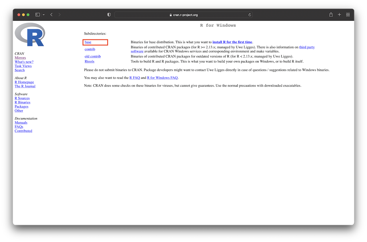
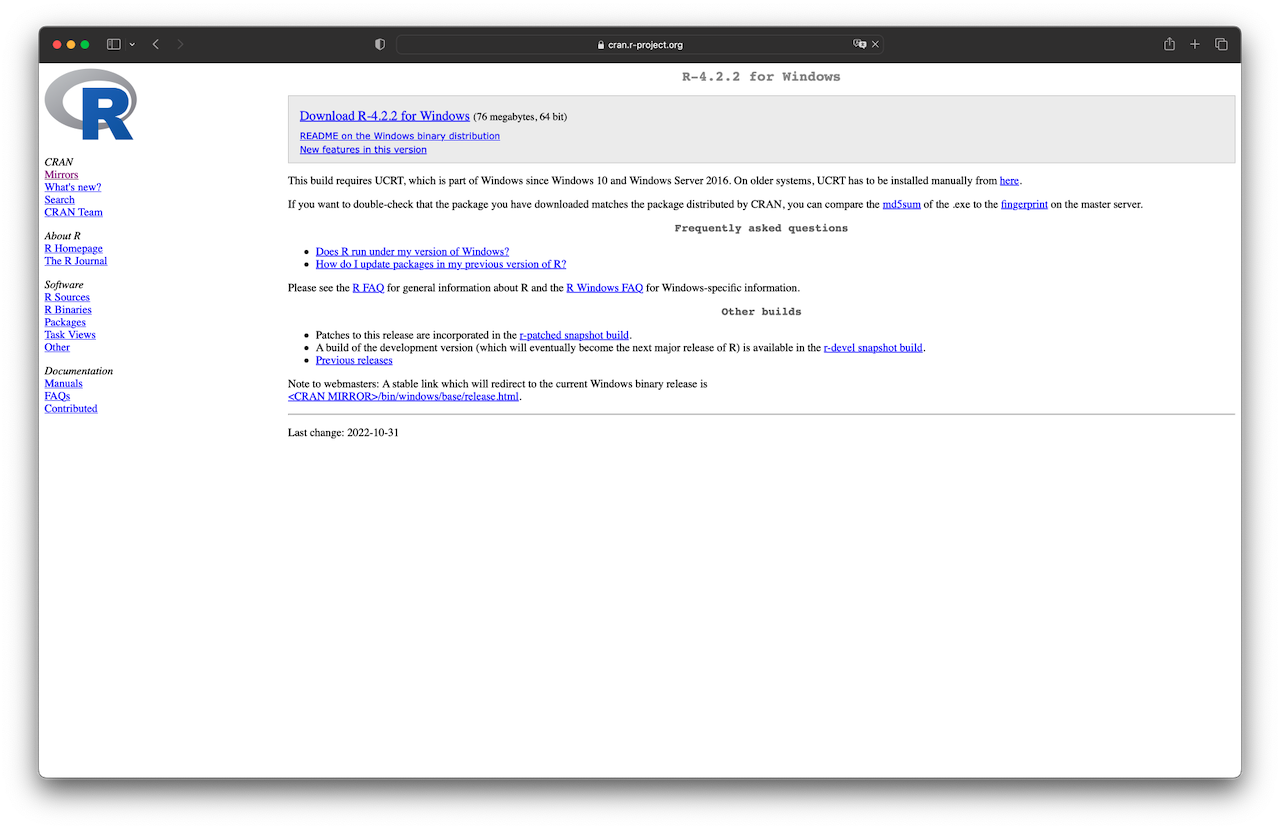
Figure 1.2: Download R for Windows.

For macOS users, click “Download R for macOS.” This will take you to a screen similar to Figure 1.3. Then, depending on your computer, click “R-4.3.2.pkg” for Mac computers with Intel processors or “R-4.3.2-arm64.pkg” for Mac computers with Apple silicon. This will download an installation file. Finally, open the file and follow the installation steps.

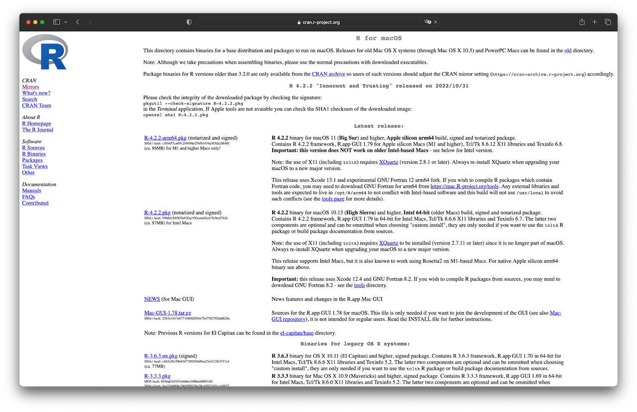
Figure 1.3: Download R for macOS.

If you followed the steps above, you should be able to open R. When starting R, a screen similar to Figure 1.4 should appear.

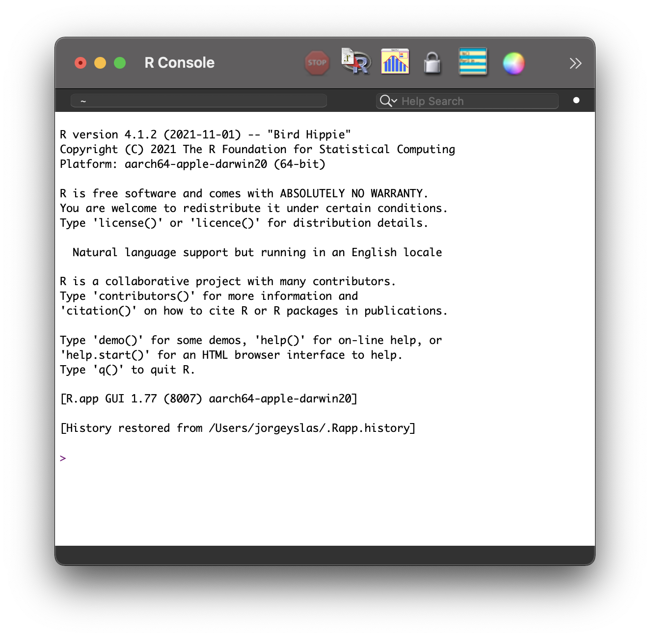
Figure 1.4: R console.

Remark. The steps above refer to version 4.3.2 of R, which corresponds to the most recent version at the time of writing. However, you should download the most current release of R.

1.1.2 Installation of Rstudio

Although the editor of R works fairly well, you should consider running R with RStudio. We will use RStudio here because it makes using R much easier and gives you access to many useful functionalities. For instance, these lecture notes were written using Rstudio. To download your copy, go to the Rstudio download page https://posit.co/download/rstudio-desktop/. Then, scroll down and click “DOWNLOAD RSTUDIO DESKTOP FOR MAC (WINDOWS)” under the heading “Step 2: Install RStudio Desktop” (see Figure 1.5), which will download the installer recommended according to your system. If the system suggested is incorrect, you can select the appropriate one from the installers list. Then, download the installation file, open it, and follow the installation steps.

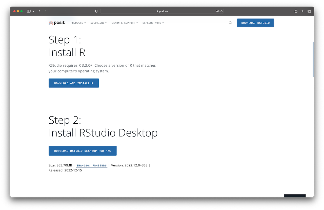
Figure 1.5: Download Rstudio.

Test the installation by opening Rstudio. You should see a screen similar to Figure 1.6.

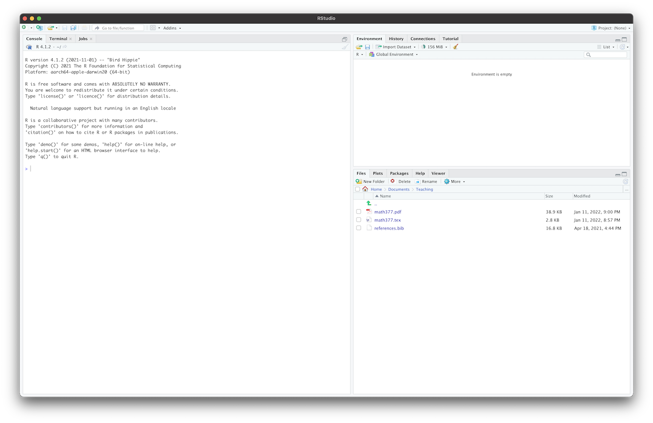
Figure 1.6: Rstudio.

Remark. Note that even if you use RStudio, you still need to download and install R. RStudio runs the version of R installed on your computer, and it does not come with a version of R on its own.

1.2 R as a simple calculator

We will start by using R as a calculator. To run R code, go to the console tab (bottom left in the default Rstudio arrangement). You will see a > symbol called the prompt. Now, type 1 + 2 after the prompt and press Enter. RStudio will display the following:

> 1 + 2
[1] 3

The [1] that appears next to our result indicates that the line starts with the first value in our result. Some commands return more than one value, and their results may show up in multiple lines. For instance, type the command 10:50, which produces 51 integer values from 10 to 50. As a result, you will see something like the following:

> 10:50
[1] 10 11 12 13 14 15 16 17 18 19 20 21 22 23 24 25 26 27 28 29 30 31 32
[24] 33 34 35 36 37 38 39 40 41 42 43 44 45 46 47 48 49 50

Here, [24] indicates that the second line starts with the 24th value. We will come back to the : operator later.

If we type an incomplete command and hit Enter, R will display a + prompt. This means that R is waiting for the rest of our command. At this stage, we can finish the command and press Enter or hit the Escape key to start over.

> 2 - 
+ 3 +
+ 5
[1] 4

In what follows, the code will be shown in this way:

1 + 2

## [1] 3

Note that we no longer display the prompt and that the results are presented after two hashtags (##). The reason is that this makes it easier for you to copy and paste the code into your R console.

Returning to using R as a calculator, Table 1.1 shows the arithmetic operators available in R.

Table 1.1: Arithmetic operators.
Addition	+
Subtraction	-
Multiplication	*
Division	/
Power	^
Integer division	%/%
Modulus (remainder of integer division)	%%

Lets now try some simple operations:

3^2 + 4 * 10

## [1] 49

(3^2 + 4) * 10

## [1] 130

One needs to be aware that the precedence for arithmetic operators in R follows the BODMAS order: Brackets ( ), Orders ^, Division / and Multiplication *, Addition +, and Subtraction -.

Remark. If you want to learn more about how R gives precedence to all operators, type ?Syntax in the console.

If we make a mistake in your code, R will let us know and indicate what the error is.

3 + *

## Error: <text>:1:5: unexpected '*'
## 1: 3 + *
##         ^

Example 1.1 Find the present value of an investment that gives 1 in 5 years, assuming that the interest rate is $r=3\%$ compounded annually.

Solution. $\,$

(1 + 0.03)^(-5)

## [1] 0.8626088

R also has several common constants and mathematical functions. These include the exponential and log functions exp() and log(), and trigonometry functions such as sin() and cos(), among others.

pi

## [1] 3.141593

cos(2 * pi)

## [1] 1

log(10) # The default option is base e

## [1] 2.302585

We can look at the full description of a function in R by using the “help.” Let us try this with the log() function. For this, we need type help(log) or ?log. This will display the documentation of the log() function in the tab Help (bottom right). Here, we will find out that log() computes the natural logarithm by default. Moreover, looking at the rest of the documentation, we will see that log() has, in fact, two arguments: x and base, the latter with the default value of the mathematical constant $e$. When calling this function, we can specify the argument names. In such a case, then the order does not matter:

log(x = 4, base = 10)

## [1] 0.60206

log(base = 10, x = 4)

## [1] 0.60206

However, if we do not specify the argument names, R will decide that x is the first argument and base is the second one.

log(4, 10)

## [1] 0.60206

log(10, 4)

## [1] 1.660964

If we try to do an operation that is not mathematically defined, R will return NaN (Not a Number).

log(-2)

## Warning in log(-2): NaNs produced

## [1] NaN

0 / 0

## [1] NaN

1.2.1 Logical operators

Logical operators help evaluate certain conditions. For instance, we may be interested in checking if an insurance claim is greater than (>) a given deductible. If this is “true,” then the insurance company may pay the amount above the deductible. Table 1.2 displays a list of logical operators in R. These operators return a Boolean value of either TRUE or FALSE.

Table 1.2: Logical operators.
Less Than	<
Less Than or Equal To	<=
Greater Than	>
Greater Than or Equal To	>=
Equal To	==
Not Equal To	!=
Not	!
Or	\|
And	&

Following, we have some simple examples:

4 <= 3

## [1] FALSE

1 == 1

## [1] TRUE

(3 != 2) & !(1 > 1)

## [1] TRUE

1.3 R objects

An essential part of any programming language is the ability to store information in variables. R lets us save data by storing it inside an R object. An object is just a name that you can use to call up stored data. First, we need to see how to create objects.

1.3.1 Assignment

Objects in R are created using the assignment operator <-, that is, the less than symbol, <, followed by a minus sign, -. Simply choose a name followed by <- and the information you want to store. For example:

x <- 1

Our variable will now be part of what is called the “working space.” We can print the value stored in this variable by typing its name

## [1] 1

or, alternatively, we can use the print() function

print(x)

## [1] 1

We need to make sure that the assignment operator is well-written. Otherwise, we may obtain an error:

x < -1

## Error in eval(expr, envir, enclos): object 'x' not found

There are a few rules regarding the name of an object in R. First, a name cannot start with a number. Second, a name cannot use some special symbols, like ^, !, $, @, +, -, /, or *. Other than that, we can name our variables in any way we want. However, it is convenient to choose a name that will help us (and others) easily read our code. Note also that R is also case-sensitive. This means that in the following code, the variables my_variable and My_variable are different objects:

my_variable <- 1
My_variable <- 2
my_variable

## [1] 1

If we use a name that is already taken, R will overwrite any previous information stored in that object:

x <- 3
x

## [1] 3

x <- 10
x

## [1] 10

Hence, it is good to check if the names we will use are already taken. We can see which object names we have already used with the function ls() or in the Environment tab of Rstudio:

ls()

## [1] "my_variable" "My_variable" "x"

We also need to be careful not to use the name of a function or constant that is already in R. This can lead to hard-to-identify errors or incorrect outputs:

pi <- 10 

sin(2 * pi)

## [1] 0.9129453

To remove specific objects from the working space, we can use the rm() function:

rm(my_variable)
ls()

## [1] "My_variable" "pi"          "x"

This can also be done using the RStudio interface. We need to ensure the Environment tab is in Grid (not List) mode, tick the object(s) we want to remove from the environment and click the broom icon.

To clean the whole working space, we type

rm(list = ls())
ls()

## character(0)

or click the broom icon in the Environment tab (List mode) in Rstudio.

Remark. Objects can also be created using = instead of <-. Although = is simpler to type, we do not recommend using it since it will make your code more difficult to read. Alternatively, one can use the shortcut alt/opt + - to generate <-.

Just as we performed calculations with numbers in the previous section, we can do the same with objects containing number references. Let us come back to Example 1.1. An alternative solution using objects would be as follows:

maturity <- 5
r <- 0.03
(1 + r)^(-maturity)

## [1] 0.8626088

As our analysis gets more complicated, we may want to save the results to access them later:

pv <- (1 + r)^(-maturity)
pv

## [1] 0.8626088

For instance, if we now want to compute the present value of an investment that gives 75 at the end of 5 years (assuming the same 3% interest rate), we can simply type:

75 * pv

## [1] 64.69566

Let us imagine that we need to repeat the analysis above, but this time using different inputs (for instance, a different interest rate). If we used the console solely, we would need to go back in the console history, change where needed, and rerun the rest of the code. This is particularly complicated when we have several lines of code. Hopefully, we can use scripts to avoid this situation. To open a new script, go to File -> New File -> R script. This will open a new script. Here, we can write our code and run it afterward using shortcuts such as Cmd+Enter or using the Run button in Rstudio.

1.3.2 Data types

R has different types of variables. These are some of the most commonly used:

Numeric - Any number in $\mathbb{R}$.
Complex - Complex numbers ($\mathbb{C}$)
Character - Collection of characters. For instance, the name of a student.
Logical - TRUE and FALSE

A difference between R and other programming languages, such as C++, is that we can declare a variable without specifying its type. Instead, R will automatically determine the type.

Numeric

R is equipped with useful functions that can be used to find the type of a variable. For instance, the class() function:

x <- log(2)
x

## [1] 0.6931472

class(x)

## [1] "numeric"

We can also check if a variable is of a certain type. For instance, the function is.numeric() checks whether a variable is of the numeric type and returns a boolean value accordingly.

is.numeric(x)

## [1] TRUE

R can store data only up to a certain point. This means that, for instance, $\pi$, which has an infinite decimal representation, is computed up to a finite number of decimal points. This is the reason why expressions such as the next one do not give exactly 0 as a result:

exp(log(10)) - 10

## [1] 1.776357e-15

R has a special command to represent infinity: Inf. We can check which is the largest number below Inf using:

.Machine$double.xmax

## [1] 1.797693e+308

Any number above this will be converted to Inf.

2e+308

## [1] Inf

We can use logical operators to check if a number is below Inf.

2e+308 < Inf

## [1] FALSE

2e+306 < Inf

## [1] TRUE

Remark. The above notation using e is to specify scientific notation in R. For instance,

2e+2 # This corresponds to 2 * 10^2

## [1] 200

3.5e-1 # This corresponds to 3.5 * 10^(-1)

## [1] 0.35

Inf can also be used in calculations and to represent certain quantities:

1 / 0

## [1] Inf

1 / Inf

## [1] 0

Remark. It is possible to work with integers in R. To specify that a number is an integer, we need to type L after the number:

x <- 2L
class(x)

## [1] "integer"

However, integers can easily be converted to numeric objects when performing computations. Hence, it is very likely that one will never need to work with integers.

y <- 1 * x
class(y)

## [1] "numeric"

Complex

A complex number is specified by adding the suffix i.

x <- -3i
x

## [1] 0-3i

class(x)

## [1] "complex"

We need to make sure to include a number before i. Otherwise, R will try to look for an object.

x <- i

## Error in eval(expr, envir, enclos): object 'i' not found

The order of real and complex parts does not matter.

x <- 2 - 1i
x

## [1] 2-1i

y <- -1i + 2
y

## [1] 2-1i

We can check if a variable is complex using the is.complex() function:

is.complex(x)

## [1] TRUE

is.numeric(x)

## [1] FALSE

We can also perform calculations with this type of objects:

x + y

## [1] 4-2i

R has some built-in functions to transform the type of data. For instance, we could use as.numeric() to try to transform a complex into a numeric

as.numeric(x)

## Warning: imaginary parts discarded in coercion

## [1] 2

Note that a warning message is displayed, indicating that R only took the real part.

Character

A character string is specified by using quotation marks (").

x <- "Hello world"
x

## [1] "Hello world"

class(x)

## [1] "character"

We can use single (') or double (") quotes, but not a mix.

x <- "Actuarial"
x

## [1] "Actuarial"

y <- 'Mathematics'
y

## [1] "Mathematics"

z <- 'Mix"

## Error: <text>:1:6: unexpected INCOMPLETE_STRING
## 1: z <- 'Mix"
##          ^

To check whether an object is a character string, we can use the is.character() function.

is.character(x)

## [1] TRUE

We can concatenate two character strings by using the paste() function:

paste(x, y)

## [1] "Actuarial Mathematics"

Note that by default, paste() puts a space between the two character strings. We can change this by using the sep argument:

paste(x, y, sep = ".")

## [1] "Actuarial.Mathematics"

We can convert numeric variables into character variables by using the as.character() function.

x <- 2
as.character(x)

## [1] "2"

It is also possible to pass from character to numeric.

x <- "2"
as.numeric(x)

## [1] 2

Finally, try the following code:

x <- "Hello"
as.numeric(x)

## Warning: NAs introduced by coercion

## [1] NA

This will produce a NA (short for Not Applicable). NA is used to represent missing values, or unknown values, in R.

Logical

We have already mentioned the logical constants TRUE and FALSE, when describing logical operators. These can also be stored in an object as follows:

x <- TRUE
x

## [1] TRUE

class(x)

## [1] "logical"

Alternatively, we can use T and F:

y <- F
y

## [1] FALSE

Again, we can check if a variable is of the logical type by using is.logical():

is.logical(y)

## [1] TRUE

When converting a logical variable into a numeric variable, we will obtain 1 (TRUE) or 0 (FALSE):

as.numeric(TRUE)

## [1] 1

as.numeric(FALSE)

## [1] 0

On the other hand, we can convert a numeric variable into a logical one using the as.logical() function. In such a case, any numeric value different from 0 will be converted to TRUE and only 0 to FALSE:

as.logical(2.3)

## [1] TRUE

as.logical(0)

## [1] FALSE

When performing computation, R automatically transforms TRUE to 1 and FALSE to 0, which can be very useful.

Example 1.2 A car insurance policy covers any losses above a deductible of 80. Compute the amount the company pays if a claim for 100 is registered.

Solution. $\,$

deductible <- 80
claim <- 100
payment <- (claim > deductible) * (claim - deductible)
payment

## [1] 20

What if the claim was for 70?

deductible <- 80
claim <- 70
payment <- (claim >= deductible) * (claim - deductible)
payment

## [1] 0

1.4 Vectors

Vectors are made of a set of objects. The c() function can be used to create vectors, and it is the easiest way to define and store more than one value in R.

x <- c(0, 2, 6, -1, -5, 1)
x

## [1]  0  2  6 -1 -5  1

We can check if an object is a vector by using the function is.vector():

is.vector(x)

## [1] TRUE

In fact, we have been working with vectors (of length one) for quite some time:

y <- 2
is.vector(y)

## [1] TRUE

The c() function also allows you to give other vectors as inputs; in that case, it will concatenate the vectors.

x <- c(c(0, 2), c(6, -1), -5, 1)
x

## [1]  0  2  6 -1 -5  1

There are other ways to generate (numeric) vectors. Next, we describe how to use the rep() and seq() functions to do so. Let us start with the function rep(). The first argument in rep() is x, which is the vector we want to repeat. The next argument is times, corresponding to a vector with the number of times we desire to repeat the elements of x. The simplest example is using x and times as vectors of length one:

rep(1, 4)

## [1] 1 1 1 1

Note that in the above code, we omitted the name of the argument times, given that it is the first optional argument. Next, we can give a vector of any length as input in x and times as vectors of length one:

rep(c(1, 2), 4) # repeats c(1, 2) four times

## [1] 1 2 1 2 1 2 1 2

If in times we give a vector of length larger than one, this should coincide with the length of the vector passed on x, and it will repeat each entry of x according to the entries of times.

rep(c(1, 2), c(4, 2)) # repeats 1 four times and 2 two times

## [1] 1 1 1 1 2 2

The next optional argument is each, which should be a nonnegative integer. It indicates to rep() that each entry of x must be repeated the number of times given in each.

rep(c(1, 2), each = 3) # repeats 1 three times and 2 three times

## [1] 1 1 1 2 2 2

Finally, we also have the optional argument length.out, which specifies the length of the output.

rep(c(1, 2), each = 3, length.out = 5)

## [1] 1 1 1 2 2

Next, we will use the function seq(from, to, by, length.out) to generate sequences of numbers. Note that this function has four arguments, and the output will depend on the values provided for these arguments. For example, if we want to generate a sequence of integers from 10 to 20, we can type:

seq(from = 10, to = 20, by = 1)

##  [1] 10 11 12 13 14 15 16 17 18 19 20

Recall that if we omit the names of the arguments, R will take them in the order provided. So, the following code will give the same output as before:

seq(10, 20, 1)

##  [1] 10 11 12 13 14 15 16 17 18 19 20

As a matter of fact, if we look at the documentation of seq(), we can see that the default value of by is 1, so we can simply type:

seq(10, 20)

##  [1] 10 11 12 13 14 15 16 17 18 19 20

Sequences of integers are extensively used in R programming. That is why we have the shortcut operator : (you may remember this operator) to produce the same result:

10:20

##  [1] 10 11 12 13 14 15 16 17 18 19 20

Let us try now with a different increment:

seq(1, 5, by = 0.1)

##  [1] 1.0 1.1 1.2 1.3 1.4 1.5 1.6 1.7 1.8 1.9 2.0 2.1 2.2 2.3 2.4 2.5 2.6 2.7 2.8
## [20] 2.9 3.0 3.1 3.2 3.3 3.4 3.5 3.6 3.7 3.8 3.9 4.0 4.1 4.2 4.3 4.4 4.5 4.6 4.7
## [39] 4.8 4.9 5.0

The fourth argument, length.out, can be used to specify the number of values to generate. The increment will be adjusted accordingly to obtain precisely the given number.

seq(1, 5, length.out = 10)

##  [1] 1.000000 1.444444 1.888889 2.333333 2.777778 3.222222 3.666667 4.111111
##  [9] 4.555556 5.000000

So far, we have only created numeric vectors. However, creating vectors of the other data types is also possible.

x <- c("string1", "string2")
x

## [1] "string1" "string2"

x <- c(FALSE, TRUE)
x

## [1] FALSE  TRUE

x <- c(1 + 2i, 3 - 2i)
x

## [1] 1+2i 3-2i

We can also check the data type of a vector:

x <- c("string1", "string2")
class(x)

## [1] "character"

is.numeric(x)

## [1] FALSE

At this point, you may be wondering what happens when you mix objects. Try it for yourself:

class(c(2.5, "string"))
class(c(TRUE, 10))
class(c("string", FALSE))
class(c(2.5, 1i))

You will see that the assignment hierarchy is given as follows: character > complex > numeric > logical.

1.4.1 Accessing vector elements

To access and modify elements of a vector, we can employ []. It is important to point out that, in stark contrast to other programming languages (e.g., C++), where the vector index starts at 0, in R, the index begins at 1. Hence, if we want to access the first element of a vector, we need to write the following:

x <- c(0, 2, 6, -1, -5, 1)
x[1]

## [1] 0

This operator also allows you to change the value of that element:

x[1] <- 10
x

## [1] 10  2  6 -1 -5  1

If we try to access an element beyond the last element, we will get NA:

x[10]

## [1] NA

To obtain the size (or length) of a vector, we can use the function length():

length(x)

## [1] 6

Thus, one way to access the last element of a vector is the following:

x[length(x)]

## [1] 1

We may be interested in selecting multiple elements of a vector. There are different ways to do it, depending on what is required. Consider the vector

x <- c(0, 2, 6, -1, -5, 1)

To access the second and third elements, we can type:

x[c(2, 3)]

## [1] 2 6

To obtain the elements from positions 2 to 5, we can run the following:

x[2:5]

## [1]  2  6 -1 -5

We can use negative numbers if we require all the vector entries except for certain elements. For instance, the following code returns the whole vector without the first element:

x[-1]

## [1]  2  6 -1 -5  1

For multiple elements:

x[c(-1, -3)]

## [1]  2 -1 -5  1

x[-c(1, 3)] # equivalently

## [1]  2 -1 -5  1

It turns out that we can use logical indexing to subtract data, which is a very powerful tool. Let us start with a very simple example. Consider the vector

x <- c(0, 2, 5)

If we type

x[c(TRUE, FALSE, TRUE)]

## [1] 0 5

we can see that R selects the entries with TRUE values. Now, take again the vector

x <- c(0, 2, 6, -1, -5, 1)

We can use the logical operators to see, for example, which entries are nonnegative:

x >= 0

## [1]  TRUE  TRUE  TRUE FALSE FALSE  TRUE

Thus, if we want to subtract the nonnegative entries of that vector, we can type:

x[x >= 0]

## [1] 0 2 6 1

Alternatively, we can make use of the function which(). This function returns the indices that give TRUE to a logical object. For example,

which(x >= 0) # These are indices, not the values contained in the vector

## [1] 1 2 3 6

Hence, we can subtract the nonnegative entries of that vector as follows:

x[which(x >= 0)]

## [1] 0 2 6 1

If the length of the logical vector is different. R will “recycle” information:

x[c(TRUE, FALSE)]

## [1]  0  6 -5

# Equivalent to
x[c(TRUE, FALSE, TRUE, FALSE, TRUE, FALSE)]

## [1]  0  6 -5

There are two other special cases that are worth mentioning. If we put nothing inside [], we obtain the original vector

x[]

## [1]  0  2  6 -1 -5  1

If we put 0, then we obtain a vector of size 0, which is represented by numeric(0)

x[0]

## numeric(0)

1.4.2 Operations with vectors

Now, we will review some operations involving vectors.

Scalars and vectors

Let us start with operations between scalars (vectors of length one) and vectors.

x <- c(0, 2, 6, -1, -5, 1)
x * 2

## [1]   0   4  12  -2 -10   2

As we can see, R will return a new vector with entries, the entries of the original vector multiplied by the given scalar. In the same way, we can make other operations:

x / 4 + 2

## [1] 2.00 2.50 3.50 1.75 0.75 2.25

x^2

## [1]  0  4 36  1 25  1

2^x

## [1]  1.00000  4.00000 64.00000  0.50000  0.03125  2.00000

Scalar functions applied to vectors

If we apply a scalar function, such as exp(), abs() (absolute value), round(), etc., to a vector, R will compute such a function element-wise:

exp(x)

## [1] 1.000000e+00 7.389056e+00 4.034288e+02 3.678794e-01 6.737947e-03
## [6] 2.718282e+00

abs(x)

## [1] 0 2 6 1 5 1

Operations among vectors

We can also perform operations among vectors. The operators typically work element-wise. Let us try first with a sum:

x <- c(0, 2, 6, -1, -5, 1)
y <- c(1, -1, 2, 7, -2, 8)
x + y

## [1]  1  1  8  6 -7  9

We can try other operators:

x * y

## [1]  0 -2 12 -7 10  8

x^y

## [1]  0.00  0.50 36.00 -1.00  0.04  1.00

If the vectors are of different sizes, R will recycle information.

x <- c(0, 2, 6, -1, -5, 1)
y <- c(1, -1)
x + y

## [1]  1  1  7 -2 -4  0

# Equivalent to
x <- c(0, 2, 6, -1, -5, 1)
y <- c(1, -1, 1, -1, 1, -1)
x + y

## [1]  1  1  7 -2 -4  0

Finally, note that the * operator performs element-wise multiplication. However, when working with mathematical vectors one may want to compute the inner product. This can be done with the %*% operator:

x <- c(0, 2, 6, -1, -5, 1)
y <- c(1, -1, 2, 7, -2, 8)
x %*% y

##      [,1]
## [1,]   21

Remark. Recall that for two vectors $\mathbf{x} = (x_1, \dots ,x_n)$ and $\mathbf{y} = (y_1, \dots ,y_n)$, the inner product $<\mathbf{x}, \mathbf{y}>$ is defined as \[ <\mathbf{x}, \mathbf{y}> = \sum_{i = 1}^n x_i y_i \,. \]

Some vector functions

Data will be typically stored inside vectors. In order to analyze such data, we can make use of different R functions. For instance, Table 1.3 shows some useful functions.

Table 1.3: Some vector functions
`min()`	Minimum value in a vector
`max()`	Maximum value in a vector
`length()`	Number of elements in a vector
`sum()`	Sum of the elements in a vector
`mean()`	Mean of the elements in a vector
`median()`	Median of the elements in a vector
`var()`	Variance of the elements in vector
`sd()`	Standard deviation of the elements in

Remark. For given data $x_1, \dots ,x_n$, the mean() and var() functions compute the sample mean and variance given by \[ \bar{x} = \frac{1}{n}\sum_{i = 1}^n x_i \,, \quad s^2_{n-1} = \frac{1}{n-1}\sum_{i = 1}^n (x_i - \bar{x})^2 \,, \] respectively.

We can now compute several quantities of interest with all these functionalities at hand.

Example 1.3 Let us assume that the following insurance claims have been reported to an insurance company:

claims <- c(80, 20, 60, 55, 20.5, 100, 70, 89.9, 120)

How many claims were reported?

length(claims)

## [1] 9

How much is the total amount of claims?

sum(claims)

## [1] 615.4

For which amount are the minimum and maximum claim amounts?

min(claims)

## [1] 20

max(claims)

## [1] 120

What is the average claim amount?

mean(claims)

## [1] 68.37778

This can also be computer using the sum() and length() functions:

sum(claims) / length(claims)

## [1] 68.37778

What is the standard deviation of the claims?

sd(claims)

## [1] 33.81489

Again, this can be computed using other functions:

sqrt(sum((claims - mean(claims))^2) / (length(claims) - 1))

## [1] 33.81489

Now assume that all these claims have a deductible of 50, and the insurance company pays the difference between a claim and the deductible if the former is larger. On average, how much does the company have to pay for the claims above the deductible?

deductible <- 50
claims_to_pay <- claims[claims > deductible]
payment <- claims_to_pay - deductible
payment

## [1] 30.0 10.0  5.0 50.0 20.0 39.9 70.0

mean(payment)

## [1] 32.12857

1.5 Matrices, data frames, and lists

1.5.1 Matrices

Sometimes, we are interested in storing information in a matrix form. The simplest way to generate a matrix is to use the matrix() function. This function has different arguments (see the help - ?matrix), so let us see how to use some of these options. The main argument of matrix() is data, which should be a data vector.

x <- matrix(c(1, 2, 3, 4, 5, 6))
x

##      [,1]
## [1,]    1
## [2,]    2
## [3,]    3
## [4,]    4
## [5,]    5
## [6,]    6

Recall that R will execute the default option if no further arguments are passed. In the above case, it creates a one-column matrix. The next two arguments are nrow and ncol. These are used to define the dimension of a matrix:

x <- matrix(c(1, 2, 3, 4, 5, 6), nrow = 3, ncol = 2)
x

##      [,1] [,2]
## [1,]    1    4
## [2,]    2    5
## [3,]    3    6

y <- matrix(c(1, 2, 3, 4, 5, 6), nrow = 2, ncol = 3)
y

##      [,1] [,2] [,3]
## [1,]    1    3    5
## [2,]    2    4    6

We can omit the argument names, and R will assign the input to the arguments in the order they are defined in the function. In this case, nrow first and ncol second (again, see help - ?matrix).

x <- matrix(c(1, 2, 3, 4, 5, 6), 2, 3)
x

##      [,1] [,2] [,3]
## [1,]    1    3    5
## [2,]    2    4    6

y <- matrix(c(1, 2, 3, 4, 5, 6), 3, 2)
y

##      [,1] [,2]
## [1,]    1    4
## [2,]    2    5
## [3,]    3    6

Note that the above matrices are filled by columns (the default). If we want to change this, we can use the next argument byrow.

x <- matrix(c(1, 2, 3, 4, 5, 6), nrow = 3, ncol = 2, byrow = TRUE)
x

##      [,1] [,2]
## [1,]    1    2
## [2,]    3    4
## [3,]    5    6

y <- matrix(c(1, 2, 3, 4, 5, 6), nrow = 2, ncol = 3, byrow = TRUE)
y

##      [,1] [,2] [,3]
## [1,]    1    2    3
## [2,]    4    5    6

In these notes, we will mainly use the default option of filling by columns.

If we only specify one of the arguments, ncol or nrow, R will attempt to find the other parameter from the length of the data.

x <- matrix(c(1, 2, 3, 4, 5, 6), ncol = 2)
x

##      [,1] [,2]
## [1,]    1    4
## [2,]    2    5
## [3,]    3    6

y <- matrix(c(1, 2, 3, 4, 5, 6), nrow = 2)
y

##      [,1] [,2] [,3]
## [1,]    1    3    5
## [2,]    2    4    6

Finally, if we specified the dimensions of the matrix and provided a vector of length larger than ncol x nrow ( i.e., the number of entries of the matrix), R will cut out the last elements.

x <- matrix(c(1, 2, 3, 4, 5, 6, 7, 8), 3, 2)

## Warning in matrix(c(1, 2, 3, 4, 5, 6, 7, 8), 3, 2): data length [8] is not a
## sub-multiple or multiple of the number of rows [3]

##      [,1] [,2]
## [1,]    1    4
## [2,]    2    5
## [3,]    3    6

The last argument, dimnames, helps us give names to a matrix’s rows and columns.

x <- matrix(c(1, 2, 3, 4, 5, 6), 3, 2,
  dimnames = list(c("Row1", "Row2", "Row3"), c("Column1", "Column2"))
)
x

##      Column1 Column2
## Row1       1       4
## Row2       2       5
## Row3       3       6

Alternatively, names can be added (and modified) by using the colnames() and rownames() functions. Additionally, these functions can help to keep the code clearer.

x <- matrix(c(1, 2, 3, 4, 5, 6), nrow = 3, ncol = 2)
colnames(x) <- c("Column1", "Column2")
rownames(x) <- c("Row1", "Row2", "Row3")
x

##      Column1 Column2
## Row1       1       4
## Row2       2       5
## Row3       3       6

Remark. Sometimes, we will encounter matrices that are defined using data vectors created with the c() function applied multiple times. For instance,

x <- matrix(c(c(1, 2, 3), c(4, 5, 6)), 3, 2)
x

##      [,1] [,2]
## [1,]    1    4
## [2,]    2    5
## [3,]    3    6

The reason is that this “notation” can help to distinguish the different columns of your input, so it is easier to read and identify mistakes. Remember that c(c(1, 2, 3), c(4, 5, 6)) produces the same vector as c(1, 2, 3, 4, 5, 6).

We can verify if an object is a matrix using the is.matrix() function:

x <- matrix(c(1, 2, 3, 4, 5, 6), 3, 2)
is.matrix(x)

## [1] TRUE

y <- c(1, 2, 3)
is.matrix(y)

## [1] FALSE

Another important function for matrices is dim(). It has two functionalities. The first one is to tell the dimension of a matrix object.

x <- matrix(c(1, 2, 3, 4, 5, 6), 3, 2)
dim(x)

## [1] 3 2

If we only require the number of columns or rows, we can use the ncol() and nrow() functions:

nrow(x)

## [1] 3

ncol(x)

## [1] 2

The second functionality of dim() is transforming vectors into matrices.

x <- c(1, 2, 3, 4, 5, 6)
dim(x) <- c(3, 2)
x

##      [,1] [,2]
## [1,]    1    4
## [2,]    2    5
## [3,]    3    6

A matrix can also be obtained by first generating two or more vectors and then combining them using the cbind() or the rbind() functions. The cbind() function combines the vectors by making them columns of a new matrix:

x <- 2:5
y <- 9:6 
cbind(x, y) # Note that the columns have been named

##      x y
## [1,] 2 9
## [2,] 3 8
## [3,] 4 7
## [4,] 5 6

On the other hand, the rbind() function makes those vectors rows of a new matrix:

rbind(x, y) # Note that the rows have been named

##   [,1] [,2] [,3] [,4]
## x    2    3    4    5
## y    9    8    7    6

We can also create diagonal matrices by using the diag() function.

diag(c(1, 2, 3, 4))

##      [,1] [,2] [,3] [,4]
## [1,]    1    0    0    0
## [2,]    0    2    0    0
## [3,]    0    0    3    0
## [4,]    0    0    0    4

To create an identity matrix, we simply type:

diag(4)

##      [,1] [,2] [,3] [,4]
## [1,]    1    0    0    0
## [2,]    0    1    0    0
## [3,]    0    0    1    0
## [4,]    0    0    0    1

Accessing matrix elements

To access elements of a matrix, we can use the [] notation. This is done in a similar way as in vectors, but in this case, we have to specify the rows and columns ([row, column]).

x <- matrix(1:6, 3)
x

##      [,1] [,2]
## [1,]    1    4
## [2,]    2    5
## [3,]    3    6

x[3, 2]

## [1] 6

We can also modify these values:

x[3, 2] <- 8
x

##      [,1] [,2]
## [1,]    1    4
## [2,]    2    5
## [3,]    3    8

If we want a whole row of the matrix, we leave the second argument blank:

x[2, ]

## [1] 2 5

Similarly, for columns:

x[, 1]

## [1] 1 2 3

We can select multiple rows (or columns) using the c() function:

x[c(1, 3), ]

##      [,1] [,2]
## [1,]    1    4
## [2,]    3    8

x[c(1, 3), 2]

## [1] 4 8

Negative values can be used to discard certain rows (or columns):

x[, -2]

## [1] 1 2 3

x[-c(1, 3), -2]

## [1] 2

Additionally, we can also use logical operators to subtract data. For instance, consider the following matrix:

x <- matrix(c(c(10, -2, 3), c(8, 0, -5)), 3, 2)
x

##      [,1] [,2]
## [1,]   10    8
## [2,]   -2    0
## [3,]    3   -5

If, for example, we were required to subset the matrix in such a way that we only keep the rows with values in the first column that are nonnegative, this can be done as follows:

x[x[, 1] >= 0, ]

##      [,1] [,2]
## [1,]   10    8
## [2,]    3   -5

What about subsetting the matrix in such a way that we only keep rows that have only nonnegative in both columns:

x[x[, 1] >= 0 & x[, 2] >= 0, ]

## [1] 10  8

Finally, if our matrix has column or row names, we can use those names to subtract information:

x <- matrix(c(1, 2, 3, 4, 5, 6), nrow = 3, ncol = 2)
colnames(x) <- c("Column1", "Column2")
rownames(x) <- c("Row1", "Row2", "Row3")
x

##      Column1 Column2
## Row1       1       4
## Row2       2       5
## Row3       3       6

x["Row2", "Column1"]

## [1] 2

x[c("Row2", "Row1"), "Column1"]

## Row2 Row1 
##    2    1

Remark. In the last example, note that the output of the last command is a vector with names for its elements. We can also give names to the entries of a vector by using the names() function. For instance,

x <- c(1,2)
names(x) <- c("name1", "name2")
x

## name1 name2 
##     1     2

However, this functionality is not used very often.

Operations with matrices

Matrices behave pretty much in the same way as vectors when dealing with scalars and functions of scalars:

x <- matrix(1:6, 3)
x

##      [,1] [,2]
## [1,]    1    4
## [2,]    2    5
## [3,]    3    6

x^2 # Each element to the power 2

##      [,1] [,2]
## [1,]    1   16
## [2,]    4   25
## [3,]    9   36

exp(x) # Exp applied element-wise

##           [,1]      [,2]
## [1,]  2.718282  54.59815
## [2,]  7.389056 148.41316
## [3,] 20.085537 403.42879

When working with matrices of the same dimension, the computations will be performed element-wise:

x <- matrix(1:6, 3)
x

##      [,1] [,2]
## [1,]    1    4
## [2,]    2    5
## [3,]    3    6

y <- matrix(6:1, 3)
y

##      [,1] [,2]
## [1,]    6    3
## [2,]    5    2
## [3,]    4    1

x + y

##      [,1] [,2]
## [1,]    7    7
## [2,]    7    7
## [3,]    7    7

x^y

##      [,1] [,2]
## [1,]    1   64
## [2,]   32   25
## [3,]   81    6

Remark. We can also perform calculations between vectors and matrices. However, we need to be aware that R will recycle information to do so. For instance,

x <- matrix(1:6, 3)
y <- c(0.5, 2)
x * y

##      [,1] [,2]
## [1,]  0.5  8.0
## [2,]  4.0  2.5
## [3,]  1.5 12.0

# Equivalently
y <- matrix(rep(c(0.5, 2), 3), 3)
y

##      [,1] [,2]
## [1,]  0.5  2.0
## [2,]  2.0  0.5
## [3,]  0.5  2.0

x * y

##      [,1] [,2]
## [1,]  0.5  8.0
## [2,]  4.0  2.5
## [3,]  1.5 12.0

There are other important operations among matrices. Let us review some of them. To perform matrix multiplication, we need to use the %*% operator (remember * is an element-wise product):

x <- matrix(1:4, 2)
x

##      [,1] [,2]
## [1,]    1    3
## [2,]    2    4

y <- matrix(4:1, 2)
y

##      [,1] [,2]
## [1,]    4    2
## [2,]    3    1

x %*% y

##      [,1] [,2]
## [1,]   13    5
## [2,]   20    8

The transpose of a matrix can be computed with the t() function:

x <- matrix(1:6, 3)
x

##      [,1] [,2]
## [1,]    1    4
## [2,]    2    5
## [3,]    3    6

t(x)

##      [,1] [,2] [,3]
## [1,]    1    2    3
## [2,]    4    5    6

The inverse of a matrix can be obtained with the solve() function (we recommend checking the help for more details ?solve()):

x <- matrix(1:4, 2)
solve(x)

##      [,1] [,2]
## [1,]   -2  1.5
## [2,]    1 -0.5

x %*% solve(x) # To check the result

##      [,1] [,2]
## [1,]    1    0
## [2,]    0    1

We may also be interested in performing operations column- or row-wise. For instance, compute the mean by row (or column). To do so, we can use vector functions in conjunction with the apply(X, MARGIN, FUN, ...) function. The arguments of apply() are: X a matrix, MARGIN, which can be 1 for rows, 2 for columns, or c(1, 2) for rows and columns, and FUN the function to be applied. For instance, let us compute the mean by rows and columns:

x <- matrix(1:6, 3)
x

##      [,1] [,2]
## [1,]    1    4
## [2,]    2    5
## [3,]    3    6

apply(x, 1, mean)

## [1] 2.5 3.5 4.5

apply(x, 2, mean)

## [1] 2 5

Remark. Matrices can be seen as 2-dimensional arrays. We can create $n$-dimensional arrays by using the array() function.

x <- array(c(1:4, 11:14, 21:24), dim = c(2, 2, 3)) # We used dim for the dimensions
x

## , , 1
## 
##      [,1] [,2]
## [1,]    1    3
## [2,]    2    4
## 
## , , 2
## 
##      [,1] [,2]
## [1,]   11   13
## [2,]   12   14
## 
## , , 3
## 
##      [,1] [,2]
## [1,]   21   23
## [2,]   22   24

Access to an array’s elements is done the same way as for matrices, using [].

x[1, , ]

##      [,1] [,2] [,3]
## [1,]    1   11   21
## [2,]    3   13   23

x[, 1, ]

##      [,1] [,2] [,3]
## [1,]    1   11   21
## [2,]    2   12   22

x[, , 1]

##      [,1] [,2]
## [1,]    1    3
## [2,]    2    4

However, array objects do not have the same versatility as matrices.

1.5.2 Data frames

Matrices can store only one data type. However, we may want to save more than one type of data in a matrix-type format — for instance, students’ names and their grades. Data frames allow us to do precisely that. To create a data frame, we use the data.frame() function.

names <- c("student1", "student2", "student3", "student4")
grades <- c(90, 95, 85, 70)
students <- data.frame(names, grades)
students

##      names grades
## 1 student1     90
## 2 student2     95
## 3 student3     85
## 4 student4     70

Note that data.frame() has named the object’s columns. We can check if an R object is a data frame with the is.data.frame() function:

is.data.frame(students)

## [1] TRUE

Data frames allow access to their data via [] in the same way as matrices:

students[1, ] # Information of the first student

##      names grades
## 1 student1     90

students[, 2] # Grades

## [1] 90 95 85 70

students[2, 2] # Grade of second student

## [1] 95

students[students[, 2] > 80, ] # Students with grades above 80

##      names grades
## 1 student1     90
## 2 student2     95
## 3 student3     85

Data frames can also use the $ operator to access data in a specific column. We simply type the name of the data frame object followed by the $ operator and the column’s name. For instance,

students$grades

## [1] 90 95 85 70

Moreover, to access a specific element of that column, we can type:

students$grades[1]

## [1] 90

Alternatively, we can use the name of the column inside [] to access its data:

students[, "grades"]

## [1] 90 95 85 70

The next thing we may want to do with a data frame is to add more information. This can be done with the cbind() function. For instance,

age <- c(20, 21, 21, 19)
students <- cbind(students, age)
students

##      names grades age
## 1 student1     90  20
## 2 student2     95  21
## 3 student3     85  21
## 4 student4     70  19

Alternatively, we can use the $ operator:

students$email <- c("st1@liv.co", "st2@liv.co", "st3@liv.co", "st4@liv.co")
students

##      names grades age      email
## 1 student1     90  20 st1@liv.co
## 2 student2     95  21 st2@liv.co
## 3 student3     85  21 st3@liv.co
## 4 student4     70  19 st4@liv.co

Or even []:

students[, 5] <- c(1, 2, 3, 4)

The names of the columns can be accessed (and changed) using the function names():

names(students)

## [1] "names"  "grades" "age"    "email"  "V5"

names(students)[5] <- "id"
students

##      names grades age      email id
## 1 student1     90  20 st1@liv.co  1
## 2 student2     95  21 st2@liv.co  2
## 3 student3     85  21 st3@liv.co  3
## 4 student4     70  19 st4@liv.co  4

1.5.3 Lists

A list enables the storage of a variety of objects into a single one. In contrast to data frames, lists can contain different data types of different lengths. Lists can be generated in R using the function list().

month <- c("Jan", "Feb", "Mar")
value <- c(1.21, 1.245, 1.402)
type <- "monthly-interest-rate"
rate <- list(Month = month, Value = value, Type = type)
rate

## $Month
## [1] "Jan" "Feb" "Mar"
## 
## $Value
## [1] 1.210 1.245 1.402
## 
## $Type
## [1] "monthly-interest-rate"

The structure of a list object can also be displayed (in a more compact format) using str():

str(rate)

## List of 3
##  $ Month: chr [1:3] "Jan" "Feb" "Mar"
##  $ Value: num [1:3] 1.21 1.25 1.4
##  $ Type : chr "monthly-interest-rate"

As is the case with data frames, we can use $ to access information:

rate$Value

## [1] 1.210 1.245 1.402

rate$Month[1]

## [1] "Jan"

We can also use []. However, the notation, in this case, is slightly different:

rate[[1]] # First element of a list, in this case, the months

## [1] "Jan" "Feb" "Mar"

rate[[2]][2] # Second value

## [1] 1.245

We can add more data to a list in different ways. First, using the $ operator:

rate$Year <- 2021
str(rate)

## List of 4
##  $ Month: chr [1:3] "Jan" "Feb" "Mar"
##  $ Value: num [1:3] 1.21 1.25 1.4
##  $ Type : chr "monthly-interest-rate"
##  $ Year : num 2021

Second, using []:

rate[[5]] <- c("UK")
str(rate)

## List of 5
##  $ Month: chr [1:3] "Jan" "Feb" "Mar"
##  $ Value: num [1:3] 1.21 1.25 1.4
##  $ Type : chr "monthly-interest-rate"
##  $ Year : num 2021
##  $      : chr "UK"

Names can be handled in the same way as with data frames.

names(rate)[5] <- "Country"
str(rate)

## List of 5
##  $ Month  : chr [1:3] "Jan" "Feb" "Mar"
##  $ Value  : num [1:3] 1.21 1.25 1.4
##  $ Type   : chr "monthly-interest-rate"
##  $ Year   : num 2021
##  $ Country: chr "UK"

1.6 Functions

So far, we have been only using built-in R functions. However, R also allows us to create our own functions. The basic syntax to define a new R function is shown below:

function_name <- function(arg1, arg2, ...) {
  statement(s)
}

Let us try a very simple example first: compute the area of a circle given its radius. An implementation would be the following:

area_circle<- function(radius) {
   pi * radius^2
}

We can now call our function:

area_circle(2)

## [1] 12.56637

We now consider a slightly more complicated example: Program the density function of an exponentially distributed random variable $X$ with mean $\lambda^{-1}$, $\lambda >0$. Recall that this density function is given by \[ f(x) = \lambda \exp(-\lambda x) \,, \quad x>0 \,. \] We write $X \sim Exp(\lambda)$.

We now require two inputs for our function: the parameter $\lambda$ and the point $x$ where we evaluate the density.

den_exponential<- function(x, lambda) {
   lambda * exp(-lambda * x)
}

den_exponential(1, 0.5)

## [1] 0.3032653

When defining a function, we can give default values to the arguments. For example, let us make the default option of our exponential density the standard exponential, i.e., $\lambda = 1$:

den_exponential <- function(x, lambda = 1) {
   lambda * exp(-lambda * x)
}

Thus, if we do not provide the function with the second parameter, R will use 1.

den_exponential(1)

## [1] 0.3678794

We now give some important considerations when working with functions:

You can return the result of a function using the return() function. In our functions above, we did not make use of this function, and the reason is that, by default, R returns the result of the last evaluated expression. However, return() can be used for early returns. For instance, the function below terminates after the first line and returns 1, ignoring the second line.

dummy_function <- function(x) {
  return(1)
  x * 2
}
dummy_function(10)

## [1] 1

We can create objects inside a function, and these will be erased after executing the function.

dummy_function <- function(x) {
  z <- 10
  x * z
}
dummy_function(10)

## [1] 100

## Error in eval(expr, envir, enclos): object 'z' not found

R will look for objects in the global environment if they are not defined inside a function.

z <- 2
dummy_function <- function(x) {
  x * z 
}
dummy_function(10)

## [1] 20

z # Keeps the value of 2

## [1] 2

However, if we create an object inside a function with the same name as an object in the global environment, the function will use the object defined inside the function’s body.

z <- 2
dummy_function <- function(x) {
  z <- 5
  x * z
}
dummy_function(10)

## [1] 50

z # Keeps the value of 2

## [1] 2

R does not alter objects given as input of a function. Instead, it creates copies.

x <- c(2, 6, 1, 9)
dummy_function <- function(x) {
  x <- sort(x)
  x
}
dummy_function(x)

## [1] 1 2 6 9

## [1] 2 6 1 9

1.7 Packages

R comes with a preloaded selection of functions. However, contributors can make their functions available via an R package. In fact, you can make your function available in the form of an R package. The general way to install a package in CRAN is as follows:

install.packages("package_name")

Let us try this by installing the derivmkts package:

install.packages("derivmkts")

We can install multiple packages using c().

install.packages(c("ggplot2", "devtools"))

Once a package is installed, we need to call it using the library() command in order to access all its functionalities.

library(package_name)

For instance,

library(derivmkts)

R packages in CRAN are updated regularly with new functions, fix bugs, performance improvements, etc. To update an R package, we can use the update.packages() function. The syntax is similar to install.packages(), for instance,

update.packages(c("ggplot2", "devtools"))

If a package in CRAN is not updated regularly, it can potentially be removed from CRAN. This means that sometimes when a package has not been updated for a while, we will not be able to install it using install.packages(). Let us try, for instance, with the CASdatasets package:

install.packages("CASdatasets")

However, the source code of an older version may still be available, and we can use that to install the package using the command

install.packages(path_to_file, repos = NULL, type = "source")

where path_to_file is the location and name of the file. Following the example of CASdatasets package, it is available to download at http://cas.uqam.ca. Try to install this package from source (you may need to install the packages xts and sp first). As previously mentioned, packages in CRAN are updated regularly. This means that their functionality may change over time by adding, modifying, or even erasing functions. Fortunately, CRAN keeps an archive of previous versions of each package. Hence, the previous method can also be used to install an older version of a package.

Remark. Submitting a package to CRAN requires passing certain tests, documenting properly, and constantly updating. That is why some developers make their code available in other places, for instance, GitHub. We can install a package from almost anywhere using the devtools package. For example, to install a package in GitHub, we can use the function install_github().

A powerful characteristic of R is that it allows writing code in other computer languages, such as C++. However, this also means that some packages will require compilation for their installation. Thus, we need to set up our computer to do so. For Windows computers, we need to download and install Rtools, which can be found at the following link: https://cran.r-project.org/bin/windows/Rtools/. If you have installed version 4.3.2 of R (or any 4.3.x version), you will need RTools 4.3. Otherwise, you will need to select the version compatible with your R version. For Mac computers, we have two options: Download and install Xcode from the Apple store or install Xcode command line by running the following in the terminal

sudo xcode-select --install

In addition, some packages are written using Fortran, and this will require installing a Fortran compiler for macOS. The instructions can be found here: https://mac.r-project.org/tools/. However, installing Xcode or Xcode command line will work fine for the packages used in the present notes.

Test that your setup is working by installing the actuar package:

install.packages("actuar")

Finally, if after loading a package, we require to detach it, we can use the detach() function:

detach("package:ggplot2", unload = TRUE)

We can also remove packages from your library with the remove.packages() function:

remove.packages("ggplot2")

Remark. Installing, loading, updating, detaching, and erasing packages can also be done in the Packages tab of Rstudio.

1.8 Control Statements

1.8.1 Conditional statements

Conditional statements evaluate if a condition is TRUE and perform an action depending on the result. We start with the if statement. Its structure is as follows:

if (condition) {
  action(s) in case of TRUE
}

Below, there is a very simple example:

claim <- 50
deductible <- 40
if (claim > deductible) {
  print("Pay claim")
}

## [1] "Pay claim"

In this case, the claim is larger (>) than our deductible, so our condition is TRUE. Thus, R will execute the code contained inside {}. In this case, print “Pay claim.”

Remark. If our code after the if statement is only one line, {} can be committed. For instance, the above code could have been written as follows:

if (claim > deductible) 
  print("Pay claim")

## [1] "Pay claim"

Sometimes, we want to perform an action in case the condition is FALSE. In such a case, we can use the else statement.

if (condition) {
  action(s) in case of TRUE
} else {
  action(s) in case of FALSE
}

Here there is a simple example:

claim <- 30
deductible <- 40
if (claim > deductible) {
  print("Pay claim")
} else {
  print("Do not pay claim")
}

## [1] "Do not pay claim"

Remark. When if/else statements are simple, one can also make use of the ifelse() function:

ifelse(claim > deductible, "Pay claim", "Do not pay claim")

## [1] "Do not pay claim"

An advantage of the ifelse() function is that it can evaluate vectors.

x <- c(1, 2, 3, 4)
ifelse(x %% 2 == 0, "even", "odd")

## [1] "odd"  "even" "odd"  "even"

What if we want to evaluate several if/else conditions? We can use if else statements to do so.

if (condition1) {
  action(s) in case condition1 TRUE
} else if (condition2) {
  action(s) in case condition2 TRUE
} else {
  action(s) in case condition1 and condition2 FALSE
}

x <- 70
if (x < 50) {
  print("low number")
} else if (50 <= x & x <= 80) {
  print("medium number")
} else {
  print("high number")
}

## [1] "medium number"

1.8.2 Loop statements

Loops statements are used to repeat code. R has two loop statements: for and while.

while statements

A while statement repeats lines of code while a certain condition is TRUE, and it stops when it is FALSE. The general structure of a while loop is the following:

while (condition) {
  action(s) while the condition is TRUE
}

We now give a simple example.

Example 1.4 Compute the cumulative sum of integers from 1 to 20 using a while loop.

Solution. $\,$

sum_int <- 0
i <- 1
while (i <= 20) {
  sum_int <- sum_int + i
  i <- i + 1
}
sum_int

## [1] 210

for statements

When we know exactly how many times we need to repeat a loop, we can use a for loop. The format of this statement is given below:

for (index in vector) {
  action(s)
}

The most common way to use a for loop is in conjunction with the : operator. For instance, if we want to solve Example 1.4 with a for loop, this can be done as follows:

sum_int <- 0
for (i in 1:20) {
  sum_int <- sum_int + i # value of i changes automatically
}
sum_int

## [1] 210

However, we can use a for loop with any other vector.

capital <- 1
yr_rates <- c(0.05, 0.03, 0.02)
for (r in yr_rates) {
  capital <- capital * (1 + r)
}
capital

## [1] 1.10313

1.9 Vectorized operations

R has been thoughtfully optimized for several operations with vector (and matrix) objects. This is commonly called “vectorization” and allows you to write concise, efficient, and easy-to-read code. For instance, let us consider the element-wise sum of two vectors. This can be done as follows:

x <- 1:10
y <- 11:20
x + y

##  [1] 12 14 16 18 20 22 24 26 28 30

However, the same calculation can be done with a for loop (without vectorization):

z <- numeric(length(x))
for (i in 1:length(x)) {
  z[i] <- x[i] + y[i]
}
z

##  [1] 12 14 16 18 20 22 24 26 28 30

We can see that the first code is simpler to read and easier to implement (less typing). Well, it turns out that it is also more efficient. To see this, we need to measure the time each code takes to perform the same calculation, and we can use the microbenchmark package to do it. First, we need to install the package.

install.packages("microbenchmark")

To use the functionalities of microbenchmark, we need to convert our previous code into functions:

sum_vect <- function(x, y) {
  x + y
}

sum_no_vect <- function(x, y) {
  z <- numeric(length(x))
  for (i in 1:length(x)) {
    z[i] <- x[i] + y[i]
  }
  z
}

We now use microbenchmark() to measure the running times of the above functions:

library(microbenchmark)
x <- 1:10
y <- 11:20
microbenchmark(sum_vect(x, y), sum_no_vect(x, y), times = 10)

## Warning in microbenchmark(sum_vect(x, y), sum_no_vect(x, y), times = 10): less
## accurate nanosecond times to avoid potential integer overflows

## Unit: nanoseconds
##               expr  min   lq     mean median   uq     max neval
##     sum_vect(x, y)  205  205  36182.5    246  328  357520    10
##  sum_no_vect(x, y) 1025 1066 194844.3   1189 1476 1937291    10

We can see that the performance of the vectorized version is, on average, around 5 times (this number may vary from computer to computer) faster than the implementation using a for loop. In conclusion, we should aim to do as many vectorized operations as possible in our code.

1.10 Reading and writing data

In practice, data is commonly provided in the form of an external file. This can be a plain text file (.txt), a comma-separated values file (.csv), an MS Excel file, etc. Hence, it is necessary that we learn how to read and write data in different file formats.

1.10.1 Working directory

One concept that is fundamental for reading and writing data is the “working directory.” This is the directory where R will first look for files. To see our current working directory, we can use the getwd() function.

getwd()

If we want to change it to a different directory, this can be done with the setwd() function.

setwd("directory")

However, this can also be done using the Rstudio interface. For instance, to see our current working directory, we can go to the Files tab, click More, and then select Go to Working Directory. Suppose we want to set up a new working directory. In that case, this can be done by going to the Files tab, looking for the directory that we want as the working directory, clicking More, and then selecting Set as Working Directory. Alternatively, we can go to the Session menu, Set Working Directory, and then select one of the options available.

1.10.2 Writing data

To store data in a file, we can use the write.table() and write.csv() functions. Typically, the object to be written would be a data frame or a matrix. Hence, let us consider the following data frame:

names <- c("student1", "student2", "student3", "student4")
grades <- c(90, 95, 85, 70)
students <- data.frame(names, grades)
students

##      names grades
## 1 student1     90
## 2 student2     95
## 3 student3     85
## 4 student4     70

Now, we can use write.table() to write the data in a file. For instance, to generate a .txt file, we can use the following:

write.table(students, file = "students.txt")

This would produce a file that looks like this :

"names" "grades"
"1" "student1" 90
"2" "student2" 95
"3" "student3" 85
"4" "student4" 70

By default, write.table() separates the data with a space and includes the column and row names. We can adjust the above code to make a comma-separated values file (.csv) that does not include the row names.

write.table(students, file = "students.csv", sep = ",", row.names = FALSE)

Now the file looks like this:

"names","grades"
"student1",90
"student2",95
"student3",85
"student4",70

Since CSV files are easier to read for most programs (including MS Excel), we have a specific function to write this type of file: write.csv().

write.csv(students, file = "students.csv", row.names = FALSE)

The above code generates exactly the same CSV file as before.

1.10.3 Reading data

Reading data in the form of text can be done with the read.table() and read.csv() functions.

For example, if we now want to read the CSV file produced before, we can do it as follows:

the_students <- read.table("students.csv", header = TRUE, sep = ",") 
# Our file is comma delimited and with headers
the_students

##      names grades
## 1 student1     90
## 2 student2     95
## 3 student3     85
## 4 student4     70

With the above, the data is now inside a data frame. Alternatively, we could have used the read.csv() function:

the_students <- read.csv("students.csv", header = TRUE)

Remark. $\,$

Importing data can also be done with Rstudio. Simply click Import Dataset in the tab Environment.
To import data from Excel, perhaps the easier method is to export the worksheet that contains your data to a CSV file and then read it in R as described above. However, you can also use an R package such as readxl, which provides the function read_excel() to do so.